Convolution Explained

What is a Convolution?

To answer this question we can think of convolution as a simple operation that can be interpreted in different ways. In this post we’ll explore some mathematical contexts and applications where the convolution occours.

Probability Theory

The first place where, in general, we start seeing the convolution as you probably don’t know is in probability. Consider two discrete random variables, $X$ and $Y$, each with their own probability distribution. How can we determine the distribution of their sum, denoted as $Z = X + Y$? To be more precise, how do we define the probability that $Z$ equals a specific value, $z$, i.e., $P(Z = z) = P(X + Y = z)$?
Let’s take a moment to explore a simple problem where we want to calculate the probability of obtaining a particular sum when rolling a pair of dice, each with six faces. If we view each die as a random variable, we can represent the probability distribution of their sum in a tabular format.

	1	2	3	4	5	6
1	$\frac 1 {36}$	$\frac 1 {36}$	$\frac 1 {36}$	$\frac 1 {36}$	$\frac 1 {36}$	$\frac 1 {36}$
2	$\frac 1 {36}$	$\frac 1 {36}$	$\frac 1 {36}$	$\frac 1 {36}$	$\frac 1 {36}$	$\frac 1 {36}$
3	$\frac 1 {36}$	$\frac 1 {36}$	$\frac 1 {36}$	$\frac 1 {36}$	$\frac 1 {36}$	$\frac 1 {36}$
4	$\frac 1 {36}$	$\frac 1 {36}$	$\frac 1 {36}$	$\frac 1 {36}$	$\frac 1 {36}$	$\frac 1 {36}$
5	$\frac 1 {36}$	$\frac 1 {36}$	$\frac 1 {36}$	$\frac 1 {36}$	$\frac 1 {36}$	$\frac 1 {36}$
6	$\frac 1 {36}$	$\frac 1 {36}$	$\frac 1 {36}$	$\frac 1 {36}$	$\frac 1 {36}$	$\frac 1 {36}$

Now if we want to find for instance know what is the probability that the sum of the dices is 6, we can simply sum the elements highlighted in red

	1	2	3	4	5	6
1	$\frac 1 {36}$	$\frac 1 {36}$	$\frac 1 {36}$	$\frac 1 {36}$	$\frac 1 {36}$	$\frac 1 {36}$
2	$\frac 1 {36}$	$\frac 1 {36}$	$\frac 1 {36}$	$\frac 1 {36}$	$\frac 1 {36}$	$\frac 1 {36}$
3	$\frac 1 {36}$	$\frac 1 {36}$	$\frac 1 {36}$	$\frac 1 {36}$	$\frac 1 {36}$	$\frac 1 {36}$
4	$\frac 1 {36}$	$\frac 1 {36}$	$\frac 1 {36}$	$\frac 1 {36}$	$\frac 1 {36}$	$\frac 1 {36}$
5	$\frac 1 {36}$	$\frac 1 {36}$	$\frac 1 {36}$	$\frac 1 {36}$	$\frac 1 {36}$	$\frac 1 {36}$
6	$\frac 1 {36}$	$\frac 1 {36}$	$\frac 1 {36}$	$\frac 1 {36}$	$\frac 1 {36}$	$\frac 1 {36}$

So $P(Z = 6) = \frac 1 {36} + \frac 1 {36} + \frac 1 {36} + \frac 1 {36} + \frac 1 {36} = \frac 5 {36}$
We can formalize this idea for an outcome $z \in [1,6]$ with the following formula:
$$
P(Z = z) = \sum_{i=1}^6 P(X = i) \cdot P(Y = z-i)
$$

This idea can be extended to continuous probability distributions as well. In this case, the formula becomes:
$$
p_Z(z) = \int_{-\infty}^{+\infty}p_X(x) \cdot p_Y(z-x) \ dx
$$

These considerations are valid for $X$ and $Y$ independent random variables.

The previous equation is the convolution definition. Now, let’s visualize this operation graphically.
Imagine we have two normal distributions, $X \sim \mathcal N(0, 1)$ and $Y \sim \mathcal N (2, 1)$, then draw their sum.

We can see that the sum of these two random variables produces a distribution with the $X$ and $Y$ features combined. For instance, we have a huge peak in the region where $X$ and $Y$ have their respective peaks.

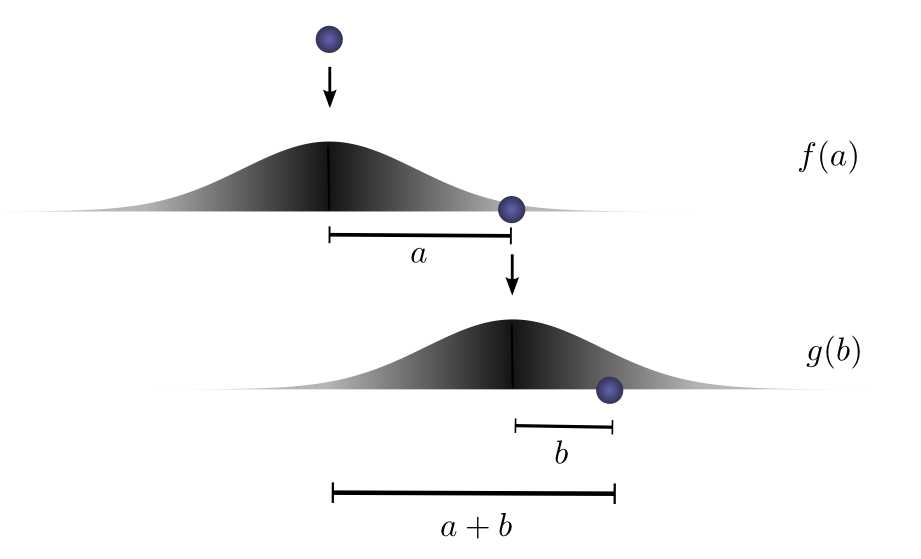
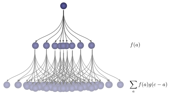
Another interesting point of view is given by Christopher Olah in this post, where we could ask what is the likelihood that a ball will travel a certain total distance $c$ after two successive drops from different heights, where each drop has its own probability distribution of distance traveled? This scenario is depicted in the image below, where $c = a + b$.

Then to get the convolution, we consider all the intermediate positions.

Digital Signal Processing

Convolution operations also find extensive use in signal processing, particularly in the context of audio signals. In audio signal processing, convolution acts as a crucial operation, functioning as a filter that operates on signal frequencies, effectively removing noise. This type of filter is referred to as a “convolutional filter,” and it can be described using the following formula:
$$
(f * g)(x) = \int_{-\infty}^{+\infty} f(t) \cdot g(x - t) dt
$$
Here, the functions $f$ and $g$ can be interpreted as our signal and the respective filter. To illustrate this concept, let’s consider a practical example of filtering an ECG (Electrocardiogram) signal using a Gaussian window filter. To confirm the removal of unwanted frequencies effectively, we can apply the Fourier transform to the filtered signal. This allows us to visualize the frequencies present in the signal, these results are displayed in the spectrum tab.

• signal
• spectrum

The convolution filter described earlier is called also stationary filter because it filters the frequencies independently for each sample in the signal. There are some more powerful filters called dynamical filters that allow us to filter the frequencies over time, using the Gabor transform.

Image Processing

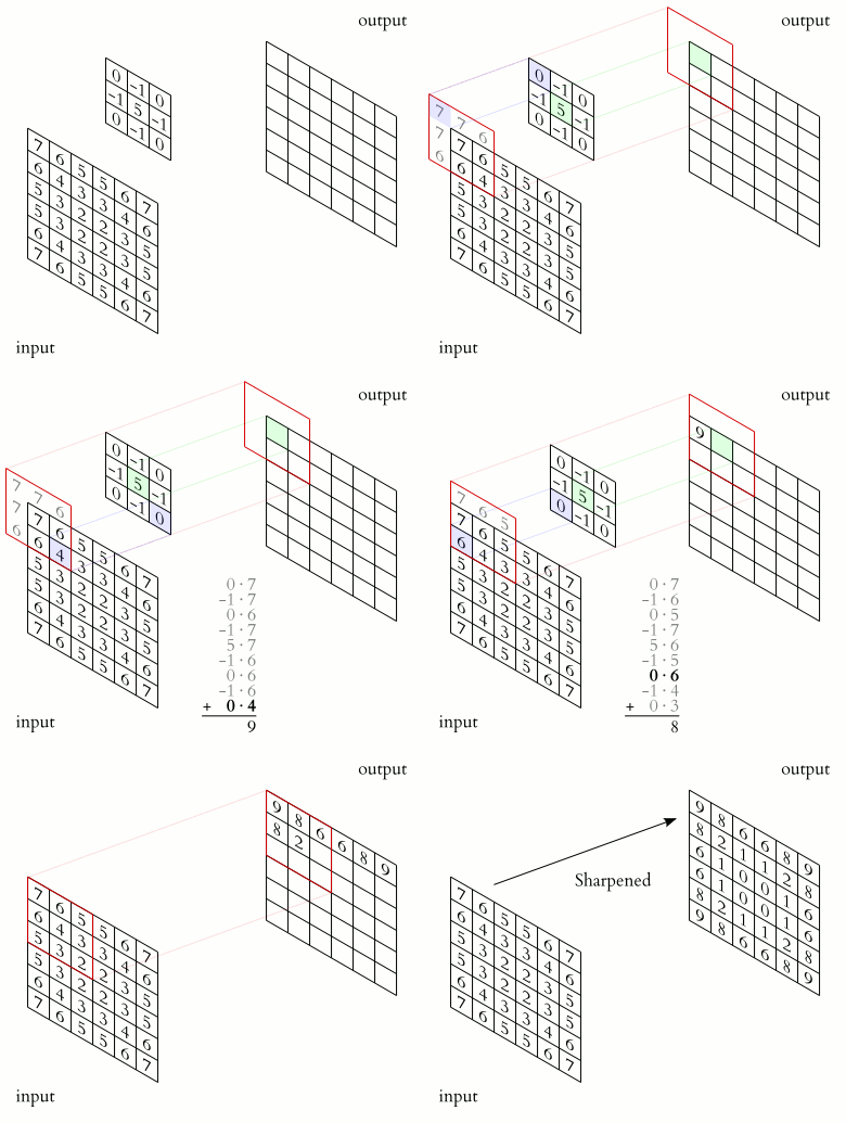
In the field of computer vision, convolutions are commonly used to apply transformations to an image, typically this is achieved using a specific kernel (filter).

Gaussian kernel

A common used kernel for blurring is the box blur kernel (also known as gaussian kernel), defined as:

$$
\frac 1 9
\begin{bmatrix}
1 & 1 & 1 \\
1 & 1 & 1 \\
1 & 1 & 1
\end{bmatrix}
$$

This specific kernel approximate the gaussian smoothing process, where we blurr an image by a gaussian function, reducing the image’s high-frequncy component, acting like a low-pass filter.

The following image summarizes the process of image convolution:

Note

In the context of deep learning, particularly in the Convolutional Neural Networks (CNNs), it’s worth noting that despite the name, the convolutional layers do not perform the convolution operation, but instead they compute an operation called cross-correlation which is very similar to convolution.

Implementation

In this section, we’ll implement the 1D convolution operation for personal preference. It’s worth noting that the implementation for 2D convolution follows a very similar approach.

import numpy as np
from math import floor, ceil
from numpy.typing import ArrayLike


def convolve(a: ArrayLike, v: ArrayLike, mode='full'):
    assert len(a.shape) == 1 and len(v.shape) == 1
    
    p = 0.0
    a_ = None
    w, k = a.shape[0], v.shape[0]
    
    match mode:
        case 'full':
            p = k - 1
            a_ = np.pad(a, pad_width=p)
        case 'valid':
            pass
        case 'same':
            p = (k-1)/2
            a_ = np.pad(a, pad_width=ceil(p))

    v_ = v[::-1]
    output_size = floor(w - k + 2 * p + 1) 
    conv = np.zeros(output_size)
    
    # do cross-correlation
    for i in range(output_size):
        conv[i] = a_[i:i+k].dot(v_)
    
    return conv

A downside of this approach is that this algorithm has a time complexity of $\mathcal O(n^2)$, making it not feasable for large number of samples. We can optimize it using the FFT algorithm, resulting in a better time complexity: $\mathcal O(n \cdot log(n))$. We can also compare our algorithm against the scipy convolution’s implementation with FFT, the results are shown in the following table.

	convolve (our implementation)	convolve (numpy)	fftconvolve (scipy)
time complexity	$\mathcal O (n^2)$	$\mathcal O (n^2)$	$\mathcal O (n\cdot log(n))$
simulation (10k)	77.7 ms	37.3 ms	3.42 ms
simulation (1M)	5.05 s	3.23 s	125 ms

We can observe that fftconvolve performs better than the naive convolution implementation, especially when dealing with a large volume of data. Additionally, it’s evident that the numpy implementation outperforms our custom one, mainly due to the fact that they have implemented the convolution routine in C.

Conclusion & Further Readings

In this post, we explored how convolution is rooted in various contexts, often interconnected. We also examined practical examples where convolution plays a crucial role. Finally we tried to implement the convolution operation for 1D signals using a naive approach. For those intrigued by an optimized approach utilizing the FFT algorithm, I recommend checking out this post.

Additionally, there are also graph convolutions, a topic we’ll delve into in future posts. These are fundamental to Graph Neural Networks (GNNs) and some of them are connected to the digital signal processing area through the Fourier transform. If you’re interested to uncover the Fourier transform and its workings, I invite you to watch this informative video.

Resources

• https://colah.github.io/posts/2014-07-Understanding-Convolutions/
• https://swharden.com/blog/2020-09-23-signal-filtering-in-python/
• https://www.youtube.com/watch?v=KuXjwB4LzSA&t=2s